Life Expectancy

We are going to be working on a linear regression model using the following dataset found on Kaggle: Countries Life Expectancy to get the toes wet with linear regression. Let's do it.

# Base imports
import numpy as np
import pandas as pd
import os

Load and Clean Data

# load data
df = pd.read_csv('/kaggle/input/countries-life-expectancy/life_expectancy.csv')
df.head(10)
Country Year Status Population Hepatitis B Measles Polio Diphtheria HIV/AIDS infant deaths under-five deaths Total expenditure GDP BMI thinness 1-19 years Alcohol Schooling Life expectancy
0 Afghanistan 2015 Developing 33736494.0 65.0 1154 6.0 65.0 0.1 62 83 8.16 584.259210 19.1 17.2 0.01 10.1 65.0
1 Afghanistan 2014 Developing 327582.0 62.0 492 58.0 62.0 0.1 64 86 8.18 612.696514 18.6 17.5 0.01 10.0 59.9
2 Afghanistan 2013 Developing 31731688.0 64.0 430 62.0 64.0 0.1 66 89 8.13 631.744976 18.1 17.7 0.01 9.9 59.9
3 Afghanistan 2012 Developing 3696958.0 67.0 2787 67.0 67.0 0.1 69 93 8.52 669.959000 17.6 17.9 0.01 9.8 59.5
4 Afghanistan 2011 Developing 2978599.0 68.0 3013 68.0 68.0 0.1 71 97 7.87 63.537231 17.2 18.2 0.01 9.5 59.2
5 Afghanistan 2010 Developing 2883167.0 66.0 1989 66.0 66.0 0.1 74 102 9.20 553.328940 16.7 18.4 0.01 9.2 58.8
6 Afghanistan 2009 Developing 284331.0 63.0 2861 63.0 63.0 0.1 77 106 9.42 445.893298 16.2 18.6 0.01 8.9 58.6
7 Afghanistan 2008 Developing 2729431.0 64.0 1599 64.0 64.0 0.1 80 110 8.33 373.361116 15.7 18.8 0.03 8.7 58.1
8 Afghanistan 2007 Developing 26616792.0 63.0 1141 63.0 63.0 0.1 82 113 6.73 369.835796 15.2 19.0 0.02 8.4 57.5
9 Afghanistan 2006 Developing 2589345.0 64.0 1990 58.0 58.0 0.1 84 116 7.43 272.563770 14.7 19.2 0.03 8.1 57.3
df.shape
(2848, 18)
# find null values
null_counts = df.isnull().sum()
null_counts
Country                   0
Year                      0
Status                    0
Population              644
Hepatitis B             542
Measles                   0
Polio                    19
Diphtheria               19
HIV/AIDS                  0
infant deaths             0
under-five deaths         0
Total expenditure       221
GDP                     442
BMI                      32
thinness  1-19 years     32
Alcohol                 188
Schooling               160
Life expectancy           0
dtype: int64

Checking where Data is null or nan

df.isnull().sum()
Country                   0
Year                      0
Status                    0
Population              644
Hepatitis B             542
Measles                   0
Polio                    19
Diphtheria               19
HIV/AIDS                  0
infant deaths             0
under-five deaths         0
Total expenditure       221
GDP                     442
BMI                      32
thinness  1-19 years     32
Alcohol                 188
Schooling               160
Life expectancy           0
dtype: int64
# print the rows with null values
df[df.isnull().any(axis=1)].head(25)
Country Year Status Population Hepatitis B Measles Polio Diphtheria HIV/AIDS infant deaths under-five deaths Total expenditure GDP BMI thinness 1-19 years Alcohol Schooling Life expectancy
32 Algeria 2015 Developing 39871528.0 95.0 63 95.0 95.0 0.1 21 24 NaN 4132.762920 59.5 6.0 NaN 14.4 75.6
44 Algeria 2003 Developing 3243514.0 NaN 15374 87.0 87.0 0.1 20 23 3.60 294.335560 47.0 6.3 0.34 11.5 71.7
45 Algeria 2002 Developing 3199546.0 NaN 5862 86.0 86.0 0.1 20 23 3.73 1774.336730 46.1 6.3 0.36 11.1 71.6
46 Algeria 2001 Developing 31592153.0 NaN 2686 89.0 89.0 0.1 20 24 3.84 1732.857979 45.3 6.4 0.23 10.9 71.4
47 Algeria 2000 Developing 3118366.0 NaN 0 86.0 86.0 0.1 21 25 3.49 1757.177970 44.4 6.5 0.25 10.7 71.3
48 Angola 2015 Developing 2785935.0 64.0 118 7.0 64.0 1.9 66 98 NaN 3695.793748 23.3 8.3 NaN 11.4 52.4
57 Angola 2006 Developing 2262399.0 NaN 765 36.0 34.0 2.5 90 143 4.54 262.415149 18.2 9.8 5.84 7.2 47.7
58 Angola 2005 Developing 19552542.0 NaN 258 39.0 38.0 2.6 92 148 4.10 1443.991929 17.7 1.0 5.04 6.8 47.4
59 Angola 2004 Developing 18865716.0 NaN 29 4.0 4.0 2.5 94 152 4.71 141.868440 17.2 1.2 3.53 6.4 47.1
60 Angola 2003 Developing 1823369.0 NaN 1196 4.0 4.0 2.4 95 155 4.41 779.468356 16.8 1.4 3.49 5.9 46.8
61 Angola 2002 Developing 17572649.0 NaN 11945 37.0 41.0 2.3 96 157 3.63 711.181716 16.3 1.5 2.82 5.5 46.5
62 Angola 2001 Developing 16983266.0 NaN 9046 41.0 38.0 2.1 97 159 5.38 526.168743 15.8 1.7 2.58 5.1 45.7
63 Angola 2000 Developing 1644924.0 NaN 2219 3.0 28.0 2.0 97 160 2.79 555.296942 15.4 1.9 1.85 4.6 45.3
64 Antigua and Barbuda 2015 Developing NaN 99.0 0 86.0 99.0 0.2 0 0 NaN 13566.954100 47.7 3.3 NaN 13.9 76.4
65 Antigua and Barbuda 2014 Developing NaN 99.0 0 96.0 99.0 0.2 0 0 5.54 12888.296670 47.0 3.3 8.56 13.9 76.2
66 Antigua and Barbuda 2013 Developing NaN 99.0 0 98.0 99.0 0.2 0 0 5.33 12224.864160 46.4 3.3 8.58 13.9 76.1
67 Antigua and Barbuda 2012 Developing NaN 98.0 0 97.0 98.0 0.2 0 0 5.39 12565.441970 45.7 3.3 8.18 13.8 75.9
68 Antigua and Barbuda 2011 Developing NaN 99.0 0 99.0 99.0 0.1 0 0 5.65 11929.349910 45.1 3.3 7.84 14.1 75.7
69 Antigua and Barbuda 2010 Developing NaN 98.0 0 99.0 98.0 0.1 0 0 5.63 12126.876140 44.4 3.3 7.84 14.1 75.6
70 Antigua and Barbuda 2009 Developing NaN 98.0 0 98.0 99.0 0.1 0 0 4.86 1312.466920 43.8 3.4 7.82 14.2 75.4
71 Antigua and Barbuda 2008 Developing NaN 98.0 0 99.0 99.0 0.1 0 0 4.69 1473.319230 43.2 3.4 8.27 14.4 75.2
72 Antigua and Barbuda 2007 Developing NaN 97.0 0 98.0 99.0 0.1 0 0 4.27 14252.294520 42.6 3.4 8.64 14.5 75.0
73 Antigua and Barbuda 2006 Developing NaN 99.0 0 99.0 99.0 0.1 0 0 4.34 12724.393770 42.0 3.4 8.93 14.7 74.8
74 Antigua and Barbuda 2005 Developing NaN 99.0 0 98.0 99.0 0.1 0 0 4.41 11371.938950 41.4 3.5 8.15 0.0 74.6
75 Antigua and Barbuda 2004 Developing NaN 97.0 0 97.0 97.0 0.1 0 0 4.21 1352.837400 4.8 3.5 7.28 0.0 74.4

From the short sample above, population is missing, alcohol is missing, hep B is missing, and many more are from the below command:

df.isnull().sum()
Country                   0
Year                      0
Status                    0
Population              644
Hepatitis B             542
Measles                   0
Polio                    19
Diphtheria               19
HIV/AIDS                  0
infant deaths             0
under-five deaths         0
Total expenditure       221
GDP                     442
BMI                      32
thinness  1-19 years     32
Alcohol                 188
Schooling               160
Life expectancy           0
dtype: int64

Find out more information about the Data

We are going to try to find out more about the columns and what might be useful for training a linear regression model.

columns = df.columns.tolist()
columns
['Country',
 'Year',
 'Status',
 'Population',
 'Hepatitis B',
 'Measles',
 'Polio',
 'Diphtheria',
 'HIV/AIDS',
 'infant deaths',
 'under-five deaths',
 'Total expenditure',
 'GDP',
 'BMI',
 'thinness  1-19 years',
 'Alcohol',
 'Schooling',
 'Life expectancy']

For each of the columns, if the data in the column is of type number we are going to print out the general information for it: (mean, std, etc) and for non-numbered data columns we are going to print out all the possible items found within the dataset. One example for the latter might be for the Status column to have [Developing, Developed]

for col in columns:
    print(f"Column '{col}':")
    if pd.api.types.is_numeric_dtype(df[col]): # if column has numeric values
        print(df[col].describe())
    else: # column has string values
        print(df[col].unique())
    print()
    
Column 'Country':
['Afghanistan' 'Albania' 'Algeria' 'Angola' 'Antigua and Barbuda'
 'Argentina' 'Armenia' 'Australia' 'Austria' 'Azerbaijan' 'Bahamas'
 'Bahrain' 'Bangladesh' 'Barbados' 'Belarus' 'Belgium' 'Belize' 'Benin'
 'Bhutan' 'Bolivia (Plurinational State of)' 'Bosnia and Herzegovina'
 'Botswana' 'Brazil' 'Brunei Darussalam' 'Bulgaria' 'Burkina Faso'
 "Côte d'Ivoire" 'Cabo Verde' 'Cambodia' 'Cameroon' 'Canada'
 'Central African Republic' 'Chad' 'Chile' 'Colombia' 'Comoros' 'Congo'
 'Costa Rica' 'Croatia' 'Cuba' 'Cyprus' 'Czechia'
 "Democratic People's Republic of Korea"
 'Democratic Republic of the Congo' 'Denmark' 'Djibouti'
 'Dominican Republic' 'Ecuador' 'Egypt' 'El Salvador' 'Equatorial Guinea'
 'Eritrea' 'Estonia' 'Fiji' 'Finland' 'France' 'Gabon' 'Gambia' 'Georgia'
 'Germany' 'Ghana' 'Greece' 'Grenada' 'Guatemala' 'Guinea' 'Guinea-Bissau'
 'Guyana' 'Haiti' 'Honduras' 'Hungary' 'Iceland' 'India' 'Indonesia'
 'Iran (Islamic Republic of)' 'Iraq' 'Ireland' 'Israel' 'Italy' 'Jamaica'
 'Japan' 'Jordan' 'Kazakhstan' 'Kenya' 'Kiribati' 'Kuwait' 'Kyrgyzstan'
 "Lao People's Democratic Republic" 'Lebanon' 'Lesotho' 'Liberia' 'Libya'
 'Lithuania' 'Luxembourg' 'Madagascar' 'Malawi' 'Malaysia' 'Maldives'
 'Mali' 'Malta' 'Mauritania' 'Mauritius' 'Mexico'
 'Micronesia (Federated States of)' 'Mongolia' 'Montenegro' 'Morocco'
 'Mozambique' 'Myanmar' 'Namibia' 'Nepal' 'Netherlands' 'New Zealand'
 'Nicaragua' 'Niger' 'Nigeria' 'Norway' 'Oman' 'Pakistan' 'Panama'
 'Paraguay' 'Peru' 'Philippines' 'Poland' 'Portugal' 'Qatar'
 'Republic of Korea' 'Republic of Moldova' 'Romania' 'Russian Federation'
 'Rwanda' 'Saint Lucia' 'Saint Vincent and the Grenadines' 'Samoa'
 'Sao Tome and Principe' 'Saudi Arabia' 'Senegal' 'Serbia' 'Seychelles'
 'Sierra Leone' 'Singapore' 'Slovakia' 'Slovenia' 'Solomon Islands'
 'Somalia' 'South Africa' 'South Sudan' 'Spain' 'Sri Lanka' 'Sudan'
 'Suriname' 'Swaziland' 'Sweden' 'Switzerland' 'Syrian Arab Republic'
 'Tajikistan' 'Thailand' 'The former Yugoslav republic of Macedonia'
 'Timor-Leste' 'Togo' 'Tonga' 'Trinidad and Tobago' 'Tunisia' 'Turkey'
 'Turkmenistan' 'Uganda' 'Ukraine' 'United Arab Emirates'
 'United Kingdom of Great Britain and Northern Ireland'
 'United Republic of Tanzania' 'United States of America' 'Uruguay'
 'Uzbekistan' 'Vanuatu' 'Venezuela (Bolivarian Republic of)' 'Viet Nam'
 'Yemen' 'Zambia' 'Zimbabwe']

Column 'Year':
count    2848.000000
mean     2007.500000
std         4.610582
min      2000.000000
25%      2003.750000
50%      2007.500000
75%      2011.250000
max      2015.000000
Name: Year, dtype: float64

Column 'Status':
['Developing' 'Developed']

Column 'Population':
count    2.204000e+03
mean     1.283457e+07
std      6.196094e+07
min      3.400000e+01
25%      1.967585e+05
50%      1.391756e+06
75%      7.438947e+06
max      1.293859e+09
Name: Population, dtype: float64

Column 'Hepatitis B':
count    2306.000000
mean       81.076756
std        25.019068
min         1.000000
25%        77.000000
50%        92.000000
75%        97.000000
max        99.000000
Name: Hepatitis B, dtype: float64

Column 'Measles':
count      2848.000000
mean       2083.082163
std       10249.107207
min           0.000000
25%           0.000000
50%          16.000000
75%         336.750000
max      212183.000000
Name: Measles, dtype: float64

Column 'Polio':
count    2829.000000
mean       82.682220
std        23.434954
min         3.000000
25%        78.000000
50%        93.000000
75%        97.000000
max        99.000000
Name: Polio, dtype: float64

Column 'Diphtheria':
count    2829.000000
mean       82.451396
std        23.693936
min         2.000000
25%        78.000000
50%        93.000000
75%        97.000000
max        99.000000
Name: Diphtheria, dtype: float64

Column 'HIV/AIDS':
count    2848.000000
mean        1.756461
std         5.148935
min         0.100000
25%         0.100000
50%         0.100000
75%         0.700000
max        50.600000
Name: HIV/AIDS, dtype: float64

Column 'infant deaths':
count    2848.000000
mean       28.359902
std       117.188032
min         0.000000
25%         0.000000
50%         3.000000
75%        20.000000
max      1800.000000
Name: infant deaths, dtype: float64

Column 'under-five deaths':
count    2848.000000
mean       39.500000
std       159.800866
min         0.000000
25%         0.000000
50%         4.000000
75%        25.000000
max      2500.000000
Name: under-five deaths, dtype: float64

Column 'Total expenditure':
count    2627.000000
mean        5.935577
std         2.504439
min         0.370000
25%         4.240000
50%         5.760000
75%         7.530000
max        17.600000
Name: Total expenditure, dtype: float64

Column 'GDP':
count      2406.000000
mean       7664.398813
std       14466.241793
min           1.681350
25%         477.541713
50%        1841.086830
75%        6265.658907
max      119172.741800
Name: GDP, dtype: float64

Column 'BMI':
count    2816.000000
mean       38.503374
std        19.955485
min         1.000000
25%        19.500000
50%        43.900000
75%        56.200000
max        77.600000
Name: BMI, dtype: float64

Column 'thinness  1-19 years':
count    2816.000000
mean        4.847230
std         4.443695
min         0.100000
25%         1.600000
50%         3.300000
75%         7.125000
max        27.700000
Name: thinness  1-19 years, dtype: float64

Column 'Alcohol':
count    2660.000000
mean        4.638932
std         4.064721
min         0.010000
25%         0.930000
50%         3.785000
75%         7.810000
max        17.870000
Name: Alcohol, dtype: float64

Column 'Schooling':
count    2688.000000
mean       12.060156
std         3.320160
min         0.000000
25%        10.200000
50%        12.400000
75%        14.300000
max        20.700000
Name: Schooling, dtype: float64

Column 'Life expectancy':
count    2848.000000
mean       69.347402
std         9.528332
min        36.300000
25%        63.500000
50%        72.200000
75%        75.800000
max        89.000000
Name: Life expectancy, dtype: float64

Status column Conversion

# convert the Status column's value in the following way:
# Developing: 0, Developed: 1
df['Status'] = df['Status'].replace({'Developing': 0, 'Developed': 1})

Possible Correlations

From the below code, there doesn't seem to be a strong correlation with any of the data directly to life expectancy, perhaps because of outliers and also because this data is not cleaned yet, but maybe a sign to use a Neural Network of some sort.

df.corr(numeric_only=True)['Life expectancy']
Year                    0.169144
Status                  0.483330
Population             -0.019353
Hepatitis B             0.256613
Measles                -0.198178
Polio                   0.464366
Diphtheria              0.476795
HIV/AIDS               -0.559105
infant deaths          -0.201055
under-five deaths      -0.224903
Total expenditure       0.222788
GDP                     0.460414
BMI                     0.567650
thinness  1-19 years   -0.477009
Alcohol                 0.401553
Schooling               0.747482
Life expectancy         1.000000
Name: Life expectancy, dtype: float64

Modified Z-Score

https://www.statology.org/modified-z-score/

Looking at Poland and other countries' data, there is a lot of information that is off. For example, Measels is recorded to have multiple zero values which does not seem very representative of the real circumstances. Moreover, population and GDP also seem to have extreme outliers. For just Poland for now, let's try to minimize these errors by using the Modified Z-Score, which calculates a Z-Score based on the median of the data.

poland = df[df['Country'] == 'Poland']
poland
Country Year Status Population Hepatitis B Measles Polio Diphtheria HIV/AIDS infant deaths under-five deaths Total expenditure GDP BMI thinness 1-19 years Alcohol Schooling Life expectancy
1952 Poland 2015 1 37986412.0 96.0 0 92.0 98.0 0.1 2 2 NaN 12565.987600 61.7 1.9 NaN 16.4 77.5
1953 Poland 2014 1 3811735.0 96.0 0 94.0 98.0 0.1 2 2 6.35 14341.675000 61.1 1.9 10.71 16.4 77.3
1954 Poland 2013 1 384196.0 96.0 84 95.0 99.0 0.1 2 2 6.40 1378.549110 6.4 2.0 11.63 15.4 77.1
1955 Poland 2012 1 3863164.0 97.0 71 95.0 99.0 0.1 2 2 6.62 13145.148400 59.7 2.0 10.81 15.3 76.8
1956 Poland 2011 1 3863255.0 98.0 0 96.0 99.0 0.1 2 2 6.70 13893.187680 59.1 2.0 10.93 15.4 76.7
1957 Poland 2010 1 3842794.0 98.0 13 96.0 99.0 0.1 2 2 6.88 12599.524860 58.4 2.1 10.59 15.1 76.3
1958 Poland 2009 1 3815163.0 98.0 115 96.0 99.0 0.1 2 3 7.12 11527.593230 57.8 2.1 10.70 15.1 75.7
1959 Poland 2008 1 38125759.0 98.0 0 96.0 99.0 0.1 2 3 6.88 141.446880 57.2 2.2 11.40 15.0 75.5
1960 Poland 2007 1 381256.0 98.0 40 99.0 99.0 0.1 2 3 6.28 1126.318520 56.6 2.2 10.90 15.0 75.3
1961 Poland 2006 1 38141267.0 98.0 120 99.0 99.0 0.1 2 3 6.17 94.772600 56.0 2.3 10.40 15.0 75.2
1962 Poland 2005 1 38165445.0 98.0 13 99.0 99.0 0.1 2 3 6.20 821.251569 55.5 2.3 9.50 14.8 75.0
1963 Poland 2004 1 38182222.0 98.0 11 99.0 99.0 0.1 2 3 6.19 6681.178818 55.0 2.4 9.19 15.5 74.9
1964 Poland 2003 1 382457.0 97.0 48 98.0 99.0 0.1 3 3 6.22 5693.524160 54.5 2.4 9.06 15.3 74.7
1965 Poland 2002 1 3823364.0 98.0 34 98.0 99.0 0.1 3 3 6.32 5196.932921 54.0 2.5 8.02 15.0 74.5
1966 Poland 2001 1 3824876.0 95.0 133 98.0 98.0 0.1 3 3 5.86 4981.198619 53.6 2.5 7.74 14.7 74.2
1967 Poland 2000 1 38258629.0 99.0 77 98.0 98.0 0.1 3 4 5.50 4492.727640 53.1 2.5 8.40 14.6 73.7

Modified Z-Score for Poland's population

from scipy.stats import median_abs_deviation # MAD Calculation

# calculate median
median = np.median(poland['Population'])

# calculate mean absolute deviation
mad = median_abs_deviation(poland['Population'])

# set threshold for outlier detection
threshold = 0.6
# this threshold for population is very low compared to recommended value of 3.5

# calculate modified z-score
modified_z_score = (0.6745 * (poland['Population'] - median)) / mad

# filter the dataframe to remove outliers
filtered = poland[np.abs(modified_z_score) <= threshold]

filtered
Country Year Status Population Hepatitis B Measles Polio Diphtheria HIV/AIDS infant deaths under-five deaths Total expenditure GDP BMI thinness 1-19 years Alcohol Schooling Life expectancy
1953 Poland 2014 1 3811735.0 96.0 0 94.0 98.0 0.1 2 2 6.35 14341.675000 61.1 1.9 10.71 16.4 77.3
1955 Poland 2012 1 3863164.0 97.0 71 95.0 99.0 0.1 2 2 6.62 13145.148400 59.7 2.0 10.81 15.3 76.8
1956 Poland 2011 1 3863255.0 98.0 0 96.0 99.0 0.1 2 2 6.70 13893.187680 59.1 2.0 10.93 15.4 76.7
1957 Poland 2010 1 3842794.0 98.0 13 96.0 99.0 0.1 2 2 6.88 12599.524860 58.4 2.1 10.59 15.1 76.3
1958 Poland 2009 1 3815163.0 98.0 115 96.0 99.0 0.1 2 3 7.12 11527.593230 57.8 2.1 10.70 15.1 75.7
1965 Poland 2002 1 3823364.0 98.0 34 98.0 99.0 0.1 3 3 6.32 5196.932921 54.0 2.5 8.02 15.0 74.5
1966 Poland 2001 1 3824876.0 95.0 133 98.0 98.0 0.1 3 3 5.86 4981.198619 53.6 2.5 7.74 14.7 74.2

In this example we actually end up filtering out the correct populations of 38 million and simply

The Input Variables

For this specific model, we are going to use the following variables to predict the life expectancy:

Selecting the Input Features

As opposed to doing modified Z-score, we are simply going to pick columns that have a general trend and are not too chaotic to predict life expectancy. This way, sure we are still including outliers but they should be balanced with the rest of the data set. We remove the statistic Measles, because somtimes we would have invalid values of >1000 for the statistic: "The number of reported measles cases per 1000 people" from looking at some developing countries.

features = ['Status', 'Polio', 'Diphtheria', \
            'HIV/AIDS', 'infant deaths', \
            'under-five deaths', 'Total expenditure',\
            'BMI', 'thinness  1-19 years', \
            'Alcohol', 'Schooling']

Building a Model: Linear Regression

We are going to split up the data, then use it to train our model. Ideally, we would want to use a training set, a validation set, and then a testing set. For this example I am going to use only the training set and testing set just to get some grips. We are going to see whether or not it may cause overfitting to the model.

# use dropna to only drop na's from the features we are trying to test
df_train = df[df['Year'] <= 2012].dropna(subset=features)
df_test = df[df['Year'] > 2012].dropna(subset=features)

print(df_train.shape)
print(df_test.shape)
(2147, 18)
(334, 18)

The year 2012 produces roughly an 80 20 split of the data [87 : 13], now let's try to train it using sklearn.

Sklearn

from sklearn.linear_model import LinearRegression

linear = LinearRegression()

target = "Life expectancy"

Fit Model

LinearRegression().fit(x, y) takes input variables and tries to fit those values to the corresponding output value. This method returns a fitted estimator of the data.

linear.fit(df_train[features], df_train[target])
LinearRegression()
In a Jupyter environment, please rerun this cell to show the HTML representation or trust the notebook.
On GitHub, the HTML representation is unable to render, please try loading this page with nbviewer.org.

Predict

Now make predictions with the testing data.

predictions = linear.predict(df_test[features])
predictions
array([63.28493162, 64.27769707, 64.24859625, 75.27033822, 75.09546198,
       75.09455566, 75.67042168, 75.5674344 , 64.72692714, 64.79060448,
       73.62910063, 73.65050985, 79.21344943, 79.23629543, 72.82693221,
       72.88084677, 86.10000331, 85.86183729, 79.56071386, 79.132046  ,
       72.32717225, 69.03080151, 72.75008102, 72.78604679, 75.84212379,
       75.8650568 , 67.45418302, 67.26566414, 75.61516906, 75.3735592 ,
       76.54800706, 76.38556271, 80.84777011, 80.89375474, 69.69366366,
       72.42435932, 66.31216642, 65.61576181, 70.08576218, 69.9833968 ,
       74.48122982, 74.20373587, 74.16342442, 74.25302967, 70.37938279,
       69.99105372, 76.58132703, 75.3147985 , 73.36448854, 75.28235669,
       78.1310823 , 77.99838215, 62.64991602, 61.56493012, 70.872569  ,
       72.43673557, 68.42888699, 66.82594233, 64.97802217, 64.80220869,
       77.53687864, 77.48479044, 57.63558552, 55.83182247, 57.17589289,
       57.08545012, 77.78829449, 74.67105451, 69.22266128, 73.57817612,
       67.88597507, 67.55055629, 62.03831576, 66.4800068 , 74.44498136,
       74.35477112, 78.84277519, 78.57979455, 71.6660567 , 75.81781643,
       78.49059565, 77.43913431, 84.41378739, 83.37668892, 61.11522541,
       60.92975373, 71.17473782, 72.67477566, 73.84684464, 73.21170279,
       71.51480137, 74.44850268, 73.57589434, 73.44234334, 58.62753644,
       56.38040847, 60.09866227, 60.11637266, 78.36257985, 78.39457351,
       77.06726094, 76.76396422, 78.67210514, 78.6454721 , 77.43905014,
       77.5072683 , 66.28674908, 67.47671129, 65.02979872, 65.0881979 ,
       73.4490736 , 73.56486948, 81.2270811 , 81.07798155, 69.34626657,
       65.8439691 , 79.39576605, 79.21577675, 75.74669664, 76.13209337,
       68.47462227, 69.4284191 , 62.02441871, 62.47129517, 63.82243698,
       62.91266769, 68.5682732 , 68.55293412, 64.97910191, 65.41127171,
       68.18636685, 71.04329185, 81.07887315, 79.52767157, 75.9714915 ,
       80.83334805, 74.49902042, 70.8401859 , 70.57013197, 72.76382284,
       76.3707057 , 76.41857878, 68.31154669, 67.15413451, 83.68576647,
       83.64783531, 77.92962151, 77.82397086, 80.87711054, 81.1979738 ,
       72.57648043, 72.30601381, 78.4167785 , 77.7683826 , 74.36522602,
       74.32762524, 75.74034336, 75.77161573, 66.47520823, 65.07594091,
       72.66080086, 73.62678216, 70.71293595, 71.2146239 , 72.59992122,
       72.22583114, 66.5251915 , 66.08054518, 73.32323065, 73.28699871,
       60.97824448, 60.79887415, 62.89264576, 65.48090617, 74.41298198,
       74.49792487, 80.22905801, 80.07087462, 74.34057063, 74.32616412,
       65.21120056, 66.02124183, 64.07825827, 63.68915426, 72.54506289,
       72.22861364, 70.61863412, 70.24914773, 61.47598447, 59.37804188,
       78.6531124 , 78.48408632, 62.97346204, 59.47729302, 74.37728622,
       74.3818426 , 73.76290316, 73.24985114, 71.2718747 , 71.50463038,
       76.07162079, 73.19183159, 76.50410476, 73.47453547, 72.70717374,
       72.6456079 , 62.69643707, 61.78537158, 65.53123655, 64.59679335,
       68.31673613, 68.10024555, 69.68782951, 69.44226371, 84.09026014,
       83.02687603, 84.58032396, 84.62719607, 71.39413139, 71.2497909 ,
       57.07433471, 57.212554  , 55.03024141, 53.58639062, 79.3429749 ,
       79.10816197, 74.39877515, 74.35617183, 65.9489262 , 65.75825716,
       67.93438432, 69.54888002, 71.62850789, 69.57556582, 73.59670618,
       72.86434158, 68.82939864, 69.75723616, 80.73075505, 76.16550381,
       78.15151872, 77.43537566, 74.62927564, 74.86715198, 79.1350676 ,
       78.07372115, 75.79868318, 75.30891527, 67.28081736, 67.08158799,
       72.45679027, 72.38566758, 73.24053627, 73.28153695, 72.64336739,
       72.8636013 , 67.61071872, 69.07396875, 77.88367647, 77.16781725,
       65.38176969, 65.0393611 , 74.90250319, 74.78071558, 72.82889369,
       73.11810039, 65.39023278, 65.41898819, 78.44226457, 78.50508405,
       78.80680048, 78.77654688, 82.03745066, 81.01581952, 68.58547716,
       68.74020574, 66.75074668, 68.24725704, 83.48502883, 82.42010017,
       72.31260616, 71.97761959, 71.94697922, 71.97956388, 65.34583458,
       63.67509382, 79.94831882, 79.92443263, 79.74146321, 79.57345789,
       65.41387719, 69.33288008, 70.48249548, 70.34294422, 72.49512271,
       72.5296839 , 73.63167428, 73.74922574, 69.83907307, 69.49706754,
       68.83035928, 68.44598107, 73.33018822, 75.89818716, 71.56709598,
       71.52544512, 72.7699083 , 75.89432363, 76.15421848, 76.12622032,
       70.33586196, 70.17163129, 63.8257878 , 63.11621233, 69.18342035,
       71.59013369, 74.39637723, 71.06658623, 76.83424233, 76.75897656,
       72.20907206, 72.0332648 , 68.77446201, 68.77730286, 74.2745724 ,
       74.45026269, 69.66084003, 68.07193834, 63.28810188, 65.3195207 ,
       67.08485043, 66.21657961, 63.35835326, 61.79454959])
This gives us an array of values that we can use to understand our predictions. However, they are not fit to a particular country and we cannot really understand the error yet either. Let's try and do that.

Understand Predictions

To start to understand our predictions, we can make a new column in the testing dataframe and add in our prediction values.

df_test['Predictions'] = predictions
df_test
Country Year Status Population Hepatitis B Measles Polio Diphtheria HIV/AIDS infant deaths under-five deaths Total expenditure GDP BMI thinness 1-19 years Alcohol Schooling Life expectancy Predictions
0 Afghanistan 2015 0 33736494.0 65.0 1154 6.0 65.0 0.1 62 83 8.16 584.259210 19.1 17.2 0.01 10.1 65.0 63.284932
1 Afghanistan 2014 0 327582.0 62.0 492 58.0 62.0 0.1 64 86 8.18 612.696514 18.6 17.5 0.01 10.0 59.9 64.277697
2 Afghanistan 2013 0 31731688.0 64.0 430 62.0 64.0 0.1 66 89 8.13 631.744976 18.1 17.7 0.01 9.9 59.9 64.248596
16 Albania 2015 0 28873.0 99.0 0 99.0 99.0 0.1 0 0 6.00 3954.227830 58.0 1.2 4.60 14.2 77.8 75.270338
17 Albania 2014 0 288914.0 98.0 0 98.0 98.0 0.1 0 1 5.88 4575.763787 57.2 1.2 4.51 14.2 77.5 75.095462
... ... ... ... ... ... ... ... ... ... ... ... ... ... ... ... ... ... ... ...
2802 Yemen 2013 0 NaN 73.0 400 67.0 73.0 0.1 36 46 5.78 NaN 39.6 13.7 0.04 9.0 65.4 65.319521
2817 Zambia 2014 0 1562974.0 86.0 9 78.0 86.0 4.3 28 41 4.99 1738.882200 22.8 6.3 0.01 12.5 61.1 67.084850
2818 Zambia 2013 0 1515321.0 79.0 35 74.0 79.0 4.8 29 42 4.99 185.793359 22.3 6.4 2.41 12.5 63.0 66.216580
2833 Zimbabwe 2014 0 15411675.0 91.0 0 92.0 91.0 6.3 23 34 6.44 127.474620 31.3 5.9 6.50 10.3 59.2 63.358353
2834 Zimbabwe 2013 0 155456.0 95.0 0 95.0 95.0 6.8 25 36 6.88 111.227396 3.8 6.2 6.39 10.4 58.0 61.794550

334 rows × 19 columns

Looking at Error

We are going to use mean absolute error from sklearn to try to understand our general loss, that is our variability of our prediction to the actual value.

from sklearn.metrics import mean_absolute_error

error = mean_absolute_error(df_test[target], df_test['Predictions'])

error
3.283831410713536

From the value, we can conclude that on average we were off by about 3.28 years on the life expectancy. This isn't too bad, and perhaps including other features could help the model do better.

df_test.describe()[target]
count    334.000000
mean      71.757186
std        8.227004
min       48.100000
25%       66.000000
50%       73.800000
75%       76.800000
max       89.000000
Name: Life expectancy, dtype: float64

Also, for our target variable, the standard deviation is higher than our error which is what we want, if the error is higher then we have made a coding mistake.

Sklearn Linear Model Analysis

Let's take a look at some countries.

df_test[df_test['Country'] == 'Grenada'].loc[:, ['Country', 'Life expectancy', 'Predictions']]
Country Life expectancy Predictions
993 Grenada 73.5 75.746697
994 Grenada 73.3 76.132093
df_test[df_test['Country'] == 'Central African Republic'].loc[:, ['Country', 'Life expectancy', 'Predictions']]
Country Life expectancy Predictions
497 Central African Republic 58.0 57.635586
498 Central African Republic 49.9 55.831822
df_test[df_test['Country'] == 'Poland'].loc[:, ['Country', 'Life expectancy', 'Predictions']]
Country Life expectancy Predictions
1953 Poland 77.3 80.730755
1954 Poland 77.1 76.165504
df_test[df_test['Country'] == 'Yemen'].loc[:, ['Country', 'Life expectancy', 'Predictions']]
Country Life expectancy Predictions
2801 Yemen 65.4 63.288102
2802 Yemen 65.4 65.319521

Looking at a few examples, the model seems to be doing quite well in predicting both developed and non-developed nations' life expectancy.

# looking at r^2 correlation
from sklearn.metrics import r2_score

r2 = r2_score(df_test[target], df_test['Predictions'])

r2
0.7357140960608528
# looking at percent error
from sklearn.metrics import mean_absolute_percentage_error as mape

pe = mape(df_test[target], df_test['Predictions'])

pe
0.047400487924007015

Looking at other metrics from sklearn, the model has a decent correlation considering all the possible variables and a low percent error.

Neural Network

Now we are going to try and make predictions based on training a Neural Network. In this example, a linear regression model might be much better at making predictions based on the correlation values, however we are going to try and practice.

target = 'Life expectancy'
# use dropna to only drop na's from the features we are trying to test
df_noNA = df.copy().dropna(subset=features)

X = df_noNA[features].values # extract input features as numpy array
y = df_noNA[target].values # extract target variable as numpy array

Split the data into training and validation sets

from sklearn.model_selection import train_test_split

X_train, X_test, y_train, y_test = train_test_split(X, y, test_size=0.2, random_state=42) # random_state is a seed for randomization

Normalizing the Data

We want to normalize the data especially for a Neural Network implementation because NN's are calculated with weights and biases, so we don't want unneccessarily high values to impact the training of the model. We are going to normalize

from sklearn.preprocessing import MinMaxScaler # calculate the percentage that the data is the highest value seen

scaler = MinMaxScaler()

X_train = scaler.fit_transform(X_train)
X_test = scaler.fit_transform(X_test)

Imports

We are going to try and train a seqeuntial neural network model.

import tensorflow as tf
from tensorflow.keras import Sequential, Input
from tensorflow.keras.layers import Dense, Dropout
from tensorflow.keras.losses import MeanAbsoluteError
from tensorflow.keras.metrics import MeanSquaredError, MeanAbsolutePercentageError
from tensorflow.keras.optimizers import Adam
/opt/conda/lib/python3.10/site-packages/tensorflow_io/python/ops/__init__.py:98: UserWarning: unable to load libtensorflow_io_plugins.so: unable to open file: libtensorflow_io_plugins.so, from paths: ['/opt/conda/lib/python3.10/site-packages/tensorflow_io/python/ops/libtensorflow_io_plugins.so']
caused by: ['/opt/conda/lib/python3.10/site-packages/tensorflow_io/python/ops/libtensorflow_io_plugins.so: undefined symbol: _ZN3tsl6StatusC1EN10tensorflow5error4CodeESt17basic_string_viewIcSt11char_traitsIcEENS_14SourceLocationE']
  warnings.warn(f"unable to load libtensorflow_io_plugins.so: {e}")
/opt/conda/lib/python3.10/site-packages/tensorflow_io/python/ops/__init__.py:104: UserWarning: file system plugins are not loaded: unable to open file: libtensorflow_io.so, from paths: ['/opt/conda/lib/python3.10/site-packages/tensorflow_io/python/ops/libtensorflow_io.so']
caused by: ['/opt/conda/lib/python3.10/site-packages/tensorflow_io/python/ops/libtensorflow_io.so: undefined symbol: _ZTVN10tensorflow13GcsFileSystemE']
  warnings.warn(f"file system plugins are not loaded: {e}")

Making the Model

model = Sequential([
    Input(shape=(11,)), # list of 11 features
    Dense(units=1024, activation='relu'),
    Dense(units=512, activation='relu'),
    Dense(units=256, activation='relu'),
    Dense(units=128, activation='relu'),
    Dense(units=64, activation='relu'),
    Dense(units=32, activation='relu'),
    Dense(units=16, activation='relu'),
    Dense(units=8, activation='relu'),
    # Dropout(0.1), # drop out a random amount of data to reduce overfitting
    Dense(units=1, activation='linear')
])

model.summary()
Model: "sequential"
_________________________________________________________________
 Layer (type)                Output Shape              Param #   
=================================================================
 dense (Dense)               (None, 1024)              12288     
                                                                 
 dense_1 (Dense)             (None, 512)               524800    
                                                                 
 dense_2 (Dense)             (None, 256)               131328    
                                                                 
 dense_3 (Dense)             (None, 128)               32896     
                                                                 
 dense_4 (Dense)             (None, 64)                8256      
                                                                 
 dense_5 (Dense)             (None, 32)                2080      
                                                                 
 dense_6 (Dense)             (None, 16)                528       
                                                                 
 dense_7 (Dense)             (None, 8)                 136       
                                                                 
 dense_8 (Dense)             (None, 1)                 9         
                                                                 
=================================================================
Total params: 712,321
Trainable params: 712,321
Non-trainable params: 0
_________________________________________________________________
model.compile(optimizer=Adam(learning_rate=0.0001),
             loss=MeanAbsoluteError(),
             metrics=[MeanAbsolutePercentageError(), MeanSquaredError()])
# train the model
history = model.fit(X_train, y_train, epochs=20, batch_size=32, validation_split=0.2) # use 20% of test data as validation set
Epoch 1/20
50/50 [==============================] - 2s 14ms/step - loss: 69.2167 - mean_absolute_percentage_error: 99.8218 - mean_squared_error: 4877.5928 - val_loss: 69.2362 - val_mean_absolute_percentage_error: 99.3120 - val_mean_squared_error: 4876.4375
Epoch 2/20
50/50 [==============================] - 0s 9ms/step - loss: 65.6733 - mean_absolute_percentage_error: 94.7047 - mean_squared_error: 4402.0762 - val_loss: 56.8149 - val_mean_absolute_percentage_error: 81.5053 - val_mean_squared_error: 3284.9976
Epoch 3/20
50/50 [==============================] - 0s 9ms/step - loss: 25.0307 - mean_absolute_percentage_error: 36.4305 - mean_squared_error: 986.6920 - val_loss: 7.6860 - val_mean_absolute_percentage_error: 11.4856 - val_mean_squared_error: 98.0215
Epoch 4/20
50/50 [==============================] - 0s 9ms/step - loss: 7.0749 - mean_absolute_percentage_error: 10.7833 - mean_squared_error: 89.4413 - val_loss: 6.3862 - val_mean_absolute_percentage_error: 9.6860 - val_mean_squared_error: 76.7808
Epoch 5/20
50/50 [==============================] - 0s 8ms/step - loss: 6.3036 - mean_absolute_percentage_error: 9.7003 - mean_squared_error: 73.8503 - val_loss: 5.8327 - val_mean_absolute_percentage_error: 8.9319 - val_mean_squared_error: 65.7295
Epoch 6/20
50/50 [==============================] - 0s 9ms/step - loss: 5.8760 - mean_absolute_percentage_error: 9.0562 - mean_squared_error: 64.8024 - val_loss: 5.5459 - val_mean_absolute_percentage_error: 8.4371 - val_mean_squared_error: 59.2126
Epoch 7/20
50/50 [==============================] - 0s 9ms/step - loss: 5.5682 - mean_absolute_percentage_error: 8.5291 - mean_squared_error: 56.2544 - val_loss: 5.2605 - val_mean_absolute_percentage_error: 8.0554 - val_mean_squared_error: 50.6454
Epoch 8/20
50/50 [==============================] - 0s 9ms/step - loss: 5.3243 - mean_absolute_percentage_error: 8.1435 - mean_squared_error: 49.9371 - val_loss: 4.8453 - val_mean_absolute_percentage_error: 7.3663 - val_mean_squared_error: 43.0707
Epoch 9/20
50/50 [==============================] - 0s 9ms/step - loss: 4.8359 - mean_absolute_percentage_error: 7.3941 - mean_squared_error: 41.1963 - val_loss: 4.4967 - val_mean_absolute_percentage_error: 6.8485 - val_mean_squared_error: 35.9151
Epoch 10/20
50/50 [==============================] - 0s 8ms/step - loss: 4.5136 - mean_absolute_percentage_error: 6.8707 - mean_squared_error: 34.9522 - val_loss: 4.1677 - val_mean_absolute_percentage_error: 6.3064 - val_mean_squared_error: 30.3279
Epoch 11/20
50/50 [==============================] - 0s 9ms/step - loss: 4.1954 - mean_absolute_percentage_error: 6.3509 - mean_squared_error: 29.6154 - val_loss: 3.8370 - val_mean_absolute_percentage_error: 5.8113 - val_mean_squared_error: 24.7149
Epoch 12/20
50/50 [==============================] - 0s 9ms/step - loss: 3.8855 - mean_absolute_percentage_error: 5.8554 - mean_squared_error: 25.3315 - val_loss: 3.7191 - val_mean_absolute_percentage_error: 5.5382 - val_mean_squared_error: 22.2857
Epoch 13/20
50/50 [==============================] - 0s 8ms/step - loss: 3.5984 - mean_absolute_percentage_error: 5.4328 - mean_squared_error: 21.7603 - val_loss: 3.5193 - val_mean_absolute_percentage_error: 5.2182 - val_mean_squared_error: 19.8640
Epoch 14/20
50/50 [==============================] - 0s 9ms/step - loss: 3.4322 - mean_absolute_percentage_error: 5.1630 - mean_squared_error: 20.1962 - val_loss: 3.2097 - val_mean_absolute_percentage_error: 4.8029 - val_mean_squared_error: 16.8289
Epoch 15/20
50/50 [==============================] - 0s 10ms/step - loss: 3.2997 - mean_absolute_percentage_error: 4.9638 - mean_squared_error: 18.9865 - val_loss: 3.0712 - val_mean_absolute_percentage_error: 4.6136 - val_mean_squared_error: 15.5695
Epoch 16/20
50/50 [==============================] - 0s 9ms/step - loss: 3.2265 - mean_absolute_percentage_error: 4.8664 - mean_squared_error: 18.2191 - val_loss: 3.0738 - val_mean_absolute_percentage_error: 4.5953 - val_mean_squared_error: 15.2571
Epoch 17/20
50/50 [==============================] - 0s 9ms/step - loss: 3.1924 - mean_absolute_percentage_error: 4.8097 - mean_squared_error: 17.7822 - val_loss: 3.0391 - val_mean_absolute_percentage_error: 4.6023 - val_mean_squared_error: 16.0240
Epoch 18/20
50/50 [==============================] - 0s 10ms/step - loss: 3.1822 - mean_absolute_percentage_error: 4.7855 - mean_squared_error: 17.7882 - val_loss: 3.0257 - val_mean_absolute_percentage_error: 4.5304 - val_mean_squared_error: 14.8641
Epoch 19/20
50/50 [==============================] - 1s 10ms/step - loss: 3.0891 - mean_absolute_percentage_error: 4.6541 - mean_squared_error: 16.8374 - val_loss: 3.0023 - val_mean_absolute_percentage_error: 4.5382 - val_mean_squared_error: 15.4936
Epoch 20/20
50/50 [==============================] - 1s 11ms/step - loss: 3.0944 - mean_absolute_percentage_error: 4.6516 - mean_squared_error: 17.0993 - val_loss: 2.9974 - val_mean_absolute_percentage_error: 4.5360 - val_mean_squared_error: 15.7211

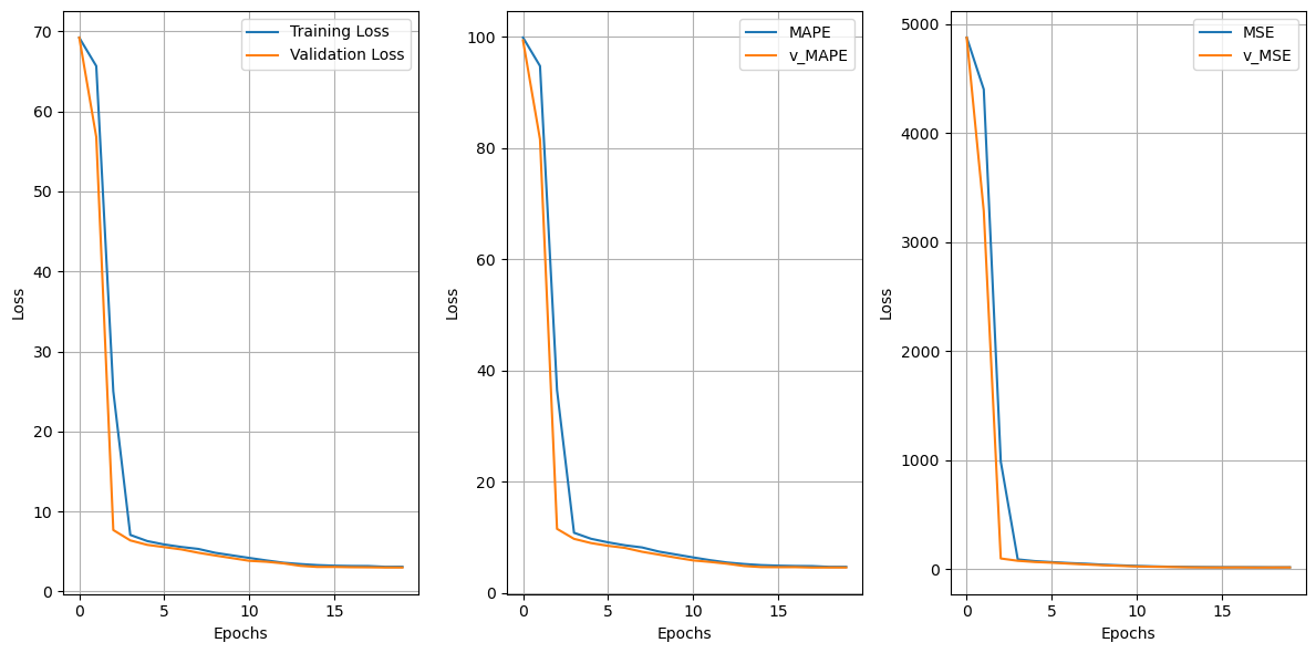
Plotting Losses

import matplotlib.pyplot as plt

# create figures
fig, axs = plt.subplots(nrows=1, ncols=3, figsize=(12, 6))

# Plot the items between the training and validation set
axs[0].plot(history.history['loss'], label='Training Loss')
axs[0].plot(history.history['val_loss'], label='Validation Loss')
axs[0].set_xlabel('Epochs')
axs[0].set_ylabel('Loss')
axs[0].legend()
axs[0].grid(True)

axs[1].plot(history.history['mean_absolute_percentage_error'], label='MAPE')
axs[1].plot(history.history['val_mean_absolute_percentage_error'], label='v_MAPE')
axs[1].set_xlabel('Epochs')
axs[1].set_ylabel('Loss')
axs[1].legend()
axs[1].grid(True)

axs[2].plot(history.history['mean_squared_error'], label='MSE')
axs[2].plot(history.history['val_mean_squared_error'], label='v_MSE')
axs[2].set_xlabel('Epochs')
axs[2].set_ylabel('Loss')
axs[2].legend()
axs[2].grid(True)

# Adjust the spacing between subplots
plt.tight_layout()

# Show the plot
plt.show()

Tweaking and messing around with the parameters of the neural network, we get a model that has a little less validation error than training error, which might be because of the nature of the problem. Let's try to run some predictions on test data. Check out this article to figure out why we might sometimes end up with a lower validation set error. Also, the difference is not too much, so we are going to assume it's a good model :thumbsup:

Making Predictions

predictions = model.predict(X_test)
16/16 [==============================] - 0s 2ms/step

Let's look at the difference between the predictions and the actual values of y_test

from sklearn.metrics import mean_absolute_error

mae = mean_absolute_error(y_test, predictions)
print(mae)
3.2141759477150993

On average with the Neural Network, we were able to predict within generally 3 years for the life expectancy, a little better but pretty much the same as the basic linear regression model which wasn't really parameterized like it maybe could be. Also, it is hard to add these values to a dataframe and compare the countries side by side. We need to know the corresponding indices. For this model, let's try and create some fun predictions:

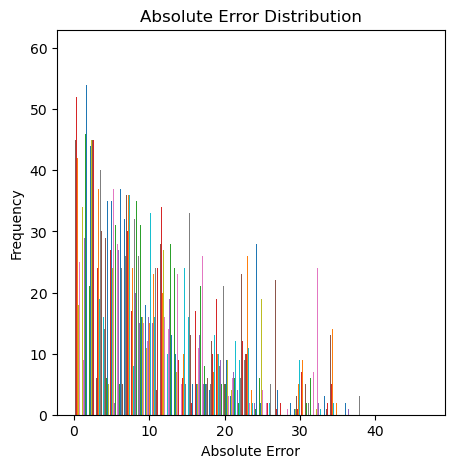
We can also plot a histogram depicting the absolute errors from their predicted values.

np.abs(predictions-y_test)
array([[ 2.7740097 ,  9.9740097 ,  0.2259903 , ...,  4.7259903 ,
         1.3740097 ,  4.9740097 ],
       [ 7.60547638,  0.40547638, 10.60547638, ..., 15.10547638,
         9.00547638,  5.40547638],
       [ 2.38466644,  9.58466644,  0.61533356, ...,  5.11533356,
         0.98466644,  4.58466644],
       ...,
       [ 8.93292236, 16.13292236,  5.93292236, ...,  1.43292236,
         7.53292236, 11.13292236],
       [ 0.3644104 ,  6.8355896 ,  3.3644104 , ...,  7.8644104 ,
         1.7644104 ,  1.8355896 ],
       [ 7.70041656, 14.90041656,  4.70041656, ...,  0.20041656,
         6.30041656,  9.90041656]])

I can't plot a histogram apparently. Unlucky.

absolute_errors = np.abs(predictions - y_test)

fig = plt.figure(figsize=(5,5))

plt.hist(absolute_errors, bins=50)

plt.title('Absolute Error Distribution')
plt.xlabel('Absolute Error')
plt.ylabel('Frequency')

plt.show()

Refresher of features: features = ['Status', 'Polio', 'Diphtheria', 'HIV/AIDS', 'infant deaths', 'under-five deaths', 'Total expenditure', 'BMI', 'thinness 1-19 years', 'Alcohol', 'Schooling']

def standardize(array):
    return scaler.transform(array) # use scaler because it is an object trained on previous data

def make_prediction(array):
    print(model.predict(array))
make_prediction(np.array([0, 0.5, 42.2131, 99.12, 4.901, 4.129, 0.15, 14.123, 78, 78, 19]).reshape(1, -1))
print(standardize(np.array([0, 0.5, 42.2131, 99.12, 4.901, 4.129, 0.15, 14.123, 78, 78, 19]).reshape(1, -1)))
1/1 [==============================] - 0s 17ms/step
[[1898.2865]]
[[ 0.00000000e+00 -2.60416667e-02  4.02243158e-01  1.96079208e+00
   2.88294118e-03  1.87681818e-03 -5.27256479e-02  1.74526749e-01
   2.86397059e+00  4.36674132e+00  9.35960591e-01]]

Ok so scaling this data and normalizing it is a little bit confusing, but we are pretty much done.

Conclusion

From this dataset, we could train 2 types of model to try and predict the life expectancy of countries. Both the linear regression from sklearn and a keras Neural Network are both effective solutions to this problem, decreasing loss on the training set and making good predictions on testing data.

EXTRA

NOT USED

Create the filtering function to go through the feature list and countries.

from scipy.stats import median_abs_deviation # MAD calculation

# for each country, modify the column as desired based on threshold
def mod_z_score(df, countries, threshold=3.5):
    new_df = pd.DataFrame(columns=features) # create empty dataframe
    for country in countries:
        if (country != 'Afghanistan'):
            new_df.reset_index(drop=True, inplace=True)
            return new_df
        
        # get the corresponding country and column information rows
        country_data = df[df['Country'] == country].dropna(subset=features) # returns DataFrame of country with no NaN's
        if len(country_data) == 0: 
            continue # if all NaN, continue to next country
        
        for feature in features:    
            # calculate median along the column
            median = np.median(country_data[feature])
            
            # calculate median absolute deviation after converting to dataframe
            mad = median_abs_deviation(country_data[feature])
            
            # calculate modified z-score
            modified_z_score = (0.6745 * (country_data[feature] - median)) / mad

            # create a mask to work around indexing errors
            mask = (np.abs(modified_z_score) <= threshold) # & (pd.notna(modified_z_score)) # (df['Country'] == country) & 
            print(mask)
            
            # filter the countries data and remove corresponding rows which don't meet the threshold
            country_data = country_data[mask]
            
        # filter the dataframe and concat it to the new object
        new_df = pd.concat([new_df, country_data])
    
    # reset the index of the new dataframe
    new_df.reset_index(drop=True, inplace=True)
    
    return new_df

# calculate with new_df = mod_z_score(df.copy(), df['Country'].unqiue().tolist())